Throughout the course, we will break out of the lecture to explore concepts more thoroughly through computational analysis. We’ll write a wide variety of code covering concepts such as mathematical techniques, stochastic simulations, and image processing. Furthermore, we will work through an experimental data set to quantify gene expression in bacterial cells.

Introductory Materials

Please work through the following tutorials before the beginning of class. The TAs will hold a special session covering these topics on Sunday, January 15th from 16:00 to 17:00 in College C.102.

• Setting up Python for scientific programming

• A primer on Python syntax and plotting

Below are links to some courses you may find useful for learning programming and data analysis in biology.

• Introduction to Programming in the Biological Sciences | A pboc-style course in which you learn practical programming in one weeks’ time.

• Data Analysis in the Biological Sciences | A wonderful course which teaches the theory and practice of Bayesian statistics using biological data. The tutorials are shown in detail in Python.

Data sets

Please download the following data sets, unzip them, and place them in your pboc/data folder as described in the setting up Python tutorial.

• Data Set 1 | A phase contrast image of bacteria and a graticule.
• Data Set 2 | A series of phase contrast and fluorescence images of a growing E. coli colony
• Data Set 3 | Images of developing fly embryos for identification of the position of the cephalic furrow.
• Data Set 4 | A large image set of E. coli strains with varying copy numbers of the lacI repressor molecule.
• Data Set 5 | An image set of 5’ and 3’ labeled mRNA expressing in the developing Drosophila embryo.

Course Python Utilities

As sometimes syntax can be difficult, we have written a file with a few functions written in Python that will make some of the in-class exercises less cumbersome. Please download them below and place them in your root pboc folder as described in the setting up Python tutorial.

• pboc_utils.py | Course utilities.

Course Exercises

As we go through the course, the code we write in class will be posted here. When possible, extra tutorials with more detail and explanation will be posted as well.

• Exercise 1 | Measuring the growth rate of E. coli cells growing on LB. [data set][in class]

• Exercise 2 | Plotting the time to diffuse a given distance. [in class]

• Exercise 3 | Plotting the analytical solution of diffusion from a delta function. [in class]

• Exercise 4 | Solving diffusion using the master equation and simulating FRAP. [in class]

• Exercise 5 | Part I of the project. We cover basic loading of images and some filtering techniques. [in class]

• Exercise 6 | Numerical integration of the mean level of transcription from a constitutive promoter. [in class]

• Exercise 7 | Solving the distribution of mRNA copy numbers through the use of a master equation. [in class]

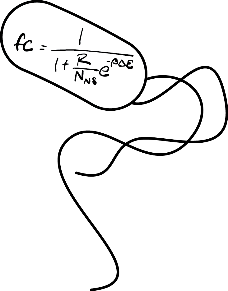
• Exercise 8 | Plotting the probabilities of the states of a simple repression promoter and exploring the fold-change. [in class]

• Exercise 9 | Part II of the project. We cover extraction of properties from fluorescent images and segmentation masks. [in class]

• Exercise 10 | Exploring the behavior of the fold-change equation considering induction of a repressor. [in class]

• Exercise 11 | We plot the nullclines of a genetic switch along with the vector fields. We also integrate in real time and show how we migrate towards the stable fixed points. [in class]

• Exercise 12 | We do some more complicated image analysis to examine the rate of transcription in the developing fly embryo. [in class] [data set]

• Exercise 13 | Part III of the project. We convert our image analysis code into functions and show the power of iteration. [in class]

• Exercise 14 | We examine how well Stirling’s approximation works for large numbers. [in class]

• Exercise 15 | We plot two theoretical predictions about phase transitions of a mixed solution. [in class]

• Exercise 16 | We ‘spread the butter’ for various modes of length control of cytoskeletal filaments. [in class]

• Exercise 17 | Part IV of the project. We perform our complete image processing pipeline over the experimental data set and test our theory of fold-change. [in class]

• Exercise 18 | We examine how genetic drift affects allele frequencies through simulation. [in class]

Extra exercises

Below are some coding exercises that were not performed in class, but are relevant to our discussions.

• Exercise 1x | Simulating diffusion as a random walk.

• Exercise 2x | Simulating the diffusion across a synapse and measuring the first passage time.