Setting Up Python For Scientific Computing
(c) 2016 Griffin Chure. This work is licensed under a Creative Commons Attribution License CC-BY 4.0. All code contained herein is licensed under an MIT license
In this tutorial, we will set up a scientific Python computing environment using the Anaconda python distribution by Continuum Analytics.
Why Python?
As is true in human language, there are hundreds of computer programming languages. While each has their own merit, the major languages for scientific computing are C, C++, R, MATLAB, Python, Java, and Fortran. MATLAB and Python are similar in syntax and typically read as if it were written in plain english. This makes both languages a useful tool for teaching but they are also very powerful languages and are very actively used in real-life research. MATLAB is proprietary while Python is open source. A benefit of being open source is that anyone can write and release Python packages. For science, there are many wonderful community-driven packages such as NumPy, SciPy, scikit-image, and Pandas just to name a few.
Installing Python 3.5 with Anaconda
Python 3.5 vs Python 2.7
There are two dominant versions of Python used for scientific computing, Python 2.7.x and Python 3.5.x. We are at an interesting crossroads between these two versions. The most recent release (Python 3.5.0 as of December 2016) is not backwards compatible with previous versions of Python. While there are still some packages written for Python 2.7 that have not been modified for compatibility with Python 3.5, a large number have transitioned. As this will be the future for scientific computing with Python, we will use Python 3.5.0 for these tutorials.
Anaconda
There are several Python distributions available for MacOS, Windows, and Linux. The two most popular, Enthought Canopy and Anaconda are specifically designed for scientific computing and data science work. For this course, we will use the Anaconda Python 3.5 distribution. To install the correct version, follow the instructions below.
- Navigate to the Anaconda download page and download the Python 3.5 graphical installer. You will be asked for your email address which you should provide. If you are affiliated with a university, you should use your
.eduaddress as you will have access to some useful goodies unavailable to the public. - Launch the installer and follow the onscreen instructions.
- Open the newly installed Anaconda Navigator application.
Congratulations! You now have the beginnings of a scientific Python distribution.
Launching an interpreter through Anaconda Navigator
Unlike MATLAB, another popular scientific computing language, Python does not have an official graphical user interface (GUI). Rather, we will be writing Python scripts in a text editor and running them through the IPython interpreter (also referred to in Anaconda as the 'qtconsole'). Here we will be able to tell our computer to execute snippets of code and run Python scripts. To launch the IPython interpreter, open the Anaconda Navigator application and click on 'Launch' under the 'qtconsole', shown in the screenshot below.

You should now be greeted with a white window with some information about your IPython version and an input prompt reading In[1]. Before we begin coding in Python, we will need to install two packages.
Installing extra packages using Conda
With the Anaconda Python distribution, you can install verified packages (scientific and non-scientific) through the Conda package manager. Note that you do not have to download Conda separately. This comes packaged with Anaconda. To install packages through Conda, we must manually enter their names on the command line. For the purposes of these tutorials, we will only need to install/upgrade two packages -- Seaborn for plotting styling and an update IPython to IPython 5.0. Rather than do this on the command line, we can install these directly from the IPython interpreter. In your IPython interpreter, type the following lines.
In[1]: ! conda upgrade ipython --yes
In[2]: ! conda install seaborn --yes
Note that the flag --yes is telling Conda that you agree to upgrade the packages on your computer that might not be compatible with other Python packages. You can remove the --yes tag, but you will have to approve them manually.
Once you have executed these commands, close the IPython interpreter window and open a new one.
Installing Atom text editor
While we now have everything we need to execute Python scripts, we need an editor to write them with. A particularly useful one is Atom, but any text editor should work. To install Atom on your machine, follow the instructions below.
Navigate to the Atom homepage and follow the instructions for installation.
Once installed, launch Atom and navigate to
Packages -> Settings View -> Openand scroll to the bottom of the page. Make sure the settingTab Lengthis set to 4. Below that, make sureTab Typeis set tosoft. This is important as indentation and white space is interpreted in Python.
Setting up the directory structure
For this course (and your coding in 'real life'), it will help if you follow a specific directory structure for your code and data. During this course, we will be writing a lot of Python scripts that will load in data. So you can directly follow along in class, it is important that you and the instructors have the same directory structure. To make this structure, open Atom and follow the instructions below.
Navigate to
File -> Add Project Folderand make a new folder in your home directory. On MacOS and Linux, this will be in/Users/YOUR_USERNAME/. On Windows, this will be XXX.Name this project
pboc.Now
pbocshould appear on the left-hand side of your editor. Right-click onpbocand make a new folder calleddata. This is where all of our data from the class will live.
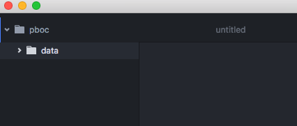
Now, if everything went well, your Atom editor window should look like this on the left-hand side.
Your first script and reading these tutorials
This tutorial (as all others in this course) are written as Jupyter notebooks which are documents which contain cells for writing text and math as well as cells that contain and excute block of Python code. While we will be writing python code in our Atom text editor, these tutorials will serve as a useful reference that not only shows the code and output, but an explaination of the biological and physical principles behind it. For these tutorials, code and it's output are rendered in two boxes as is shown below.
# This is a comment and is not read by Python
print('Hello! This is the print function. Python will print this line below')
The box with the gray background contains the python code while the output is in the box with the white background. When reading these tutorials, you may want to retype (or copy-and-paste) the code lines into Atom or in the IPython interpreter directly.
If you have followed the steps above, we are finally ready to write our first Python script. In your Atom window, create a new file named my_first_script.py and save it within your pboc root directory (not in data). You can do this by going to File -> New File then File -> Save and navigate to your pboc folder. Now, in the my_first_script.py file, we'll generate a plot of one of my favorite functions. Type (or copy and paste) the following lines into you script file and save it.
Now we are finally ready to write our first Python script. In your Atom window, create a new file named my_first_script.py and save it within your pboc root directory (not in data). You can do this by going to File -> New File then File -> Save and navigate to your pboc folder. Now, in the my_first_script.py file, we'll generate a plot of one of my favorite functions. Type (or copy and paste) the following lines into you script file and save it by going to File -> Save.
# Import Python packages necessary for this script
import numpy as np
import matplotlib.pyplot as plt
import seaborn as sns

# Generate a beautiful sinusoidal curve
x = np.linspace(0, 2*np.pi, 500)
y = np.sin(2 * np.sin(2 * np.sin(2 * x)))
plt.plot(x, y)
plt.xlabel('$x$')
plt.ylabel('$y$')
plt.show()
Once you have this file saved, open a new IPython interpreter through the Anaconda Navigator window and type the following commands.
In [1]: cd pboc
In [2]: %matplotlib
In [3]: %run my_first_script.py
The first command navigates to the correct directory. The second command allows for us to keep typing while plots are being shown. The third command runs the script we just wrote through the IPython interpreter. The percentage signs for In [2]: and In [3]: are called Python magic fuctions and are explained in the python syntax tutorial. While just typing matplotlib and run my_first_script.py will work, it is better style to use these magic functions.
If everything works as expected, you should see the plot below.
# These commands are for showing the plot in this notebook only.
%matplotlib inline
plt.plot(x, y)
plt.xlabel('$x$')
plt.ylabel('$y$')

With that, you are now set up to do some scientific computing in Python! For the rest of the course, we will be going through this same procedure to computationally explore principles of physical biology. To this end, our computer screens will typically look something like this:
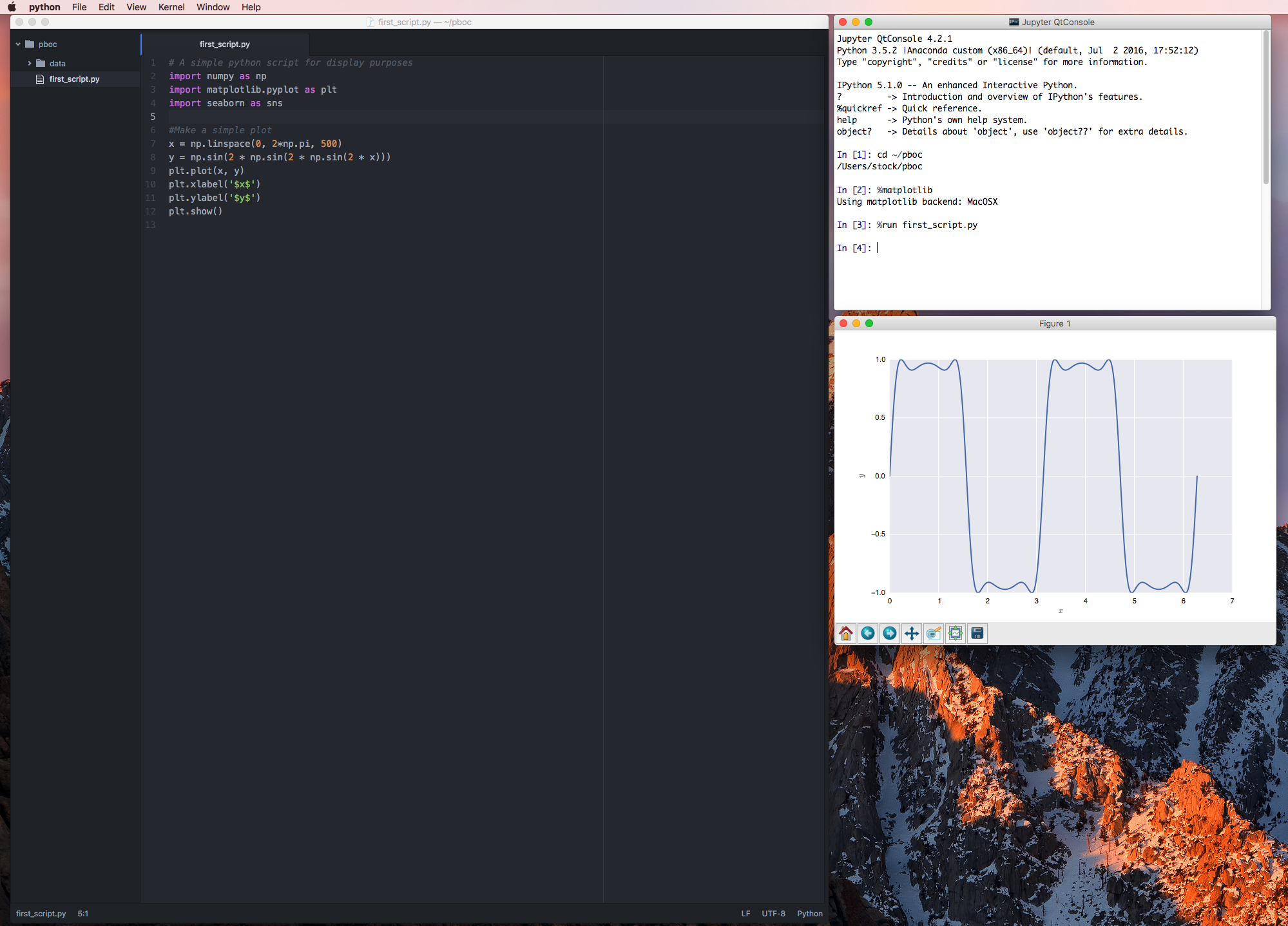
although you can code however you feel comfortable!
What is Jupyter?
Jupyter Notebooks are very useful tools for writing code, text, and math into a single document. In fact, this (and all other tutorials) were written in Jupyter noteooks. While we won't use them in this class, I strongly suggest you learn about them by following this excellent tutorial written by a Caltech Professor of Biology and Biological Engineering, Justin Bois.