Tutorial 0a: Setting Up Python For Scientific Computing
© 2018 Griffin Chure. This work is licensed under a Creative Commons Attribution License CC-BY 4.0. All code contained herein is licensed under an MIT license
In this tutorial, we will set up a scientific Python computing environment using the Anaconda python distribution by Continuum Analytics.
Why Python?
As is true in human language, there are hundreds of computer programming languages. While each has its own merit, the major languages for scientific computing are C, C++, R, MATLAB, Python, Java, and Fortran. MATLAB and Python are similar in syntax and typically read as if they were written in plain English. This makes both languages a useful tool for teaching but they are also very powerful languages and are very actively used in real-life research. MATLAB is proprietary while Python is open source. A benefit of being open source is that anyone can write and release Python packages. For science, there are many wonderful community-driven packages such as NumPy, SciPy, scikit-image, and Pandas just to name a few.
Installing Python 3.7 with Anaconda
Python 3.7 vs Python 2.7
There are two dominant versions of Python used for scientific computing, Python 2.7 and Python 3.7. We are at an interesting crossroads between these two versions. The most recent release is not backward compatible with previous versions of Python. While there are still some packages written for Python 2.7 that have not been modified for compatibility with Python 3.7, a large number have transitioned. As this will be the future for scientific computing with Python, we will use Python 3.7 for these tutorials.
Anaconda
There are several scientific Python distributions available for MacOS, Windows, and Linux. The two most popular, Enthought Canopy and Anaconda are specifically designed for scientific computing and data science work. For this course, we will use the Anaconda Python 3.7 distribution. To install the correct version, follow the instructions below.
Navigate to the Anaconda download page and download the Python 3.7 graphical installer.
Launch the installer and follow the onscreen instructions.
Congratulations! You now have the beginnings of a scientific Python distribution.
Setting up the directory structure
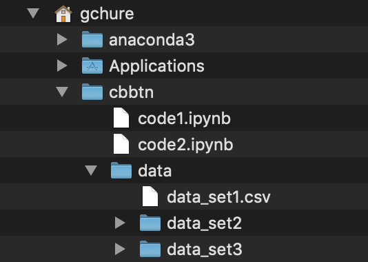
For this course (and your coding in 'real life'), it will help if you follow a specific directory structure for your code and data. During this course, we will write a lot of code that will load in data. To ensure that everyone's code runs properly, it is essential that you all set up your directories in the same way. All code we write will assume that you have the following directory structure:
In your home directory, make a new folder named
cbbtn. On MacOS and Linux, your home directory will be in/Users/YOUR_USERNAME/. On Windows, your home directory will be inC::/Users/YOUR_USERNAME/.All code files you write during the course will be saved in this
cbbtnfolder.Within the
cbbtnfolder, make a folder nameddata, into which all data files from the course will be saved.
For example, this is what my home directory structure looks like:
If you have followed all of these steps successfully, you should have a complete setup for scientific computing in Python! You are now ready to start coding! We will be using Jupyter Notebooks, which allow us to write code, text, and math into a single document. In fact, this (and all other tutorials) were written in Jupyter notebooks. The next tutorial will introduce you to Jupyter Notebooks and how to use them.