Supplemental Information
Candle
To estimate the single-cell MscL abundance via microscopy, we needed to determine a calibration factor that could translate arbitrary fluorescence units to protein copy number. To compute this calibration factor, we relied on a priori knowledge of the mean copy number of MscL-sfGFP for a particular bacterial strain in specific growth conditions. In Bialecka-Fornal et al. 2012 (1), the average MscL copy number for a population of cells expressing an MscL-sfGFP fusion (E. coli K-12 MG1655 \(\phi\)(mscL-sfGFP)) cells was measured using quantitative Western blotting and single-molecule photobleaching assays. By growing this strain in identical growth and imaging conditions, we can make an approximate measure of this calibration factor. In this section, we derive a statistical model for estimating the most-likely value of this calibration factor and its associated error.
Definition of a calibration factor
We assume that all detected fluorescence signal from a particular cell is derived from the MscL-sfGFP protein, after background subtraction and correction for autofluorescence. The arbitrary units of fluorescence can be directly related to the protein copy number via a calibration factor \(\alpha\), \[ I_\text{tot} = \alpha N_\text{tot}, \qquad(1)\] where \(I_\text{tot}\) is the total cell fluorescence and \(N_\text{tot}\) is the total number of MscL proteins per cell. Bialecka-Fornal et al. report the average cell Mscl copy number for the population rather than the distribution. Knowing only the mean, we can rewrite Eq. 1 as \[ \langle I_\text{tot}\rangle = \alpha \langle N_\text{tot} \rangle, \qquad(2)\] assuming that \(\alpha\) is a constant value that does not change from cell to cell or fluorophore to fluorophore.
The experiments presented in this work were performed using non-synchronously growing cultures. As there is a uniform distribution of growth phases in the culture, the cell size distribution is broad the the extremes being small, newborn cells and large cells in the process of division. As described in the main text, the cell size distribution of a population is broadened further by modulating the MscL copy number with low copy numbers resulting in aberrant cell morphology. To speak in the terms of an effective channel copy number, we relate the average areal intensity of the population to the average cell size, \[ \langle I_\text{tot} \rangle = \langle I_A \rangle \langle A \rangle = \alpha \langle N_\text{tot} \rangle, \qquad(3)\] where \(\langle I_A\rangle\) is the average areal intensity in arbitrary units per pixel of the population and \(\langle A \rangle\) is the average area of a segmented cell. As only one focal plane was imaged in these experiments, we could not compute an appropriate volume for each cell given the highly aberrant morphology. We therefore opted to use the projected two-dimensional area of each cell as a proxy for cell size. Given this set of measurements, the calibration factor can be computed as \[ \alpha = {\langle I_A \rangle\langle A \rangle \over \langle N_\text{tot} \rangle}. \qquad(4)\]
While it is tempting to use Eq. 4 directly, there are multiple sources of error that are important to propagate through the final calculation. The most obvious error to include is the measurement error reported in Bialecka-Fornal et al. 2012 for the average MscL channel count (1). There are also slight variations in expression across biological replicates that arise from a myriad of day-to-day differences. Rather than abstracting all sources of error away into a systematic error budget, we used an inferential model derived from Bayes' theorem that allows for the computation of the probability distribution of \(\alpha\).
Estimation of \(\alpha\) for a single biological replicate
A single data set consists of several hundred single-cell measurements of intensity, area of the segmentation mask, and other morphological quantities. The areal density \(I_A\) is computed by dividing the total cell fluorescence by the cell area \(A\). We are interested in computing the probability distributions for the calibration factor \(\alpha\), the average cell area \(\langle A \rangle\), and the mean number of channels per cell \(\langle N_\text{tot} \rangle\) for the data set as a whole given only \(I_A\) and \(A\). Using Bayes' theorem, the probability distribution for these parameters given a single cell measurement, hereafter called the posterior distribution, can be written as \[ g(\alpha, \langle A \rangle, \langle N_\text{tot} \rangle\,\vert\, A, I_A) = {f(A, I_A\,\vert \, \alpha,\langle A \rangle, \langle N_\text{tot} \rangle) g(\alpha,\langle A \rangle, \langle N_\text{tot} \rangle) \over f(\alpha, I_A)}, \qquad(5)\] where \(g\) and \(f\) represent probability density functions over parameters and data, respectively. The term \(f(A, I_A\,\vert\, \alpha, \langle A \rangle, \langle N_\text{tot} \rangle)\) in the numerator represents the likelihood of observing the areal intensity \(I_A\) and area \(A\) of a cell for a given values of \(\alpha\), \(\langle A \rangle\), and \(\langle N_\text{tot} \rangle\). The second term in the numerator \(g(\alpha,\langle A \rangle, \langle N_\text{tot} \rangle)\) captures all prior knowledge we have regarding the possible values of these parameters knowing nothing about the measured data. The denominator, \(f(I_A, A)\) captures the probability of observing the data knowing nothing about the parameter values. This term, in our case, serves simply as a normalization constant and is neglected for the remainder of this section.
To determine the appropriate functional form for the likelihood and prior, we must make some assumptions regarding the biological processes that generate them. As there are many independent processes that regulate the timing of cell division and cell growth, such as DNA replication and peptidoglycan synthesis, it is reasonable to assume that for a given culture the distribution of cell size would be normally distributed with a mean of \(\langle A \rangle\) and a variance \(\sigma_{\langle A \rangle}\). Mathematically, we can write this as \[ f(A\,\vert\,\langle A \rangle, \sigma_{\langle A \rangle}) \propto {1 \over \sigma_{\langle A \rangle}}\exp\left[-{(A - \langle A \rangle)^2 \over 2\sigma_{\langle A \rangle}^2}\right], \qquad(6)\] where the proportionality results from dropping normalization constants for notational simplicity.
While total cell intensity is intrinsically dependent on the cell area the areal intensity \(I_A\) is independent of cell size. The myriad processes leading to the detected fluorescence, such as translation and proper protein folding, are largely independent, allowing us to assume a normal distribution for \(I_A\) as well with a mean \(\langle I_A \rangle\) and a variance \(\sigma_{I_A}^2\). However, we do not have knowledge of the average areal intensity for the standard candle strain a priori. This can be calculated knowing the calibration factor, total MscL channel copy number, and the average cell area as \[ I_A = {\alpha\langle N_\text{tot} \rangle \over \langle A \rangle}. \qquad(7)\] Using Eq. 7 to calculate the expected areal intensity for the population, we can write the likelihood as a Gaussian distribution, \[ f(I_A\,\vert\,\alpha,\langle A \rangle,\langle N_\text{tot} \rangle, \sigma_{I_A}) \propto {1 \over \sigma_{I_A}}\exp\left[-{\left(I_A - {\alpha \langle N_\text{tot} \rangle\over \langle A \rangle}\right)^2 \over 2 \sigma_{I_A}^2}\right]. \qquad(8)\]
With these two likelihoods in hand, we are tasked with determining the appropriate priors. As we have assumed normal distributions for the likelihoods of \(\langle A \rangle\) and \(I_A\), we have included two additional parameters, \(\sigma_{\langle A \rangle}\) and \(\sigma_{I_A}\), each requiring their own prior probability distribution. It is common practice to assume maximum ignorance for these variances and use a Jeffreys prior (2), \[ g(\sigma_{\langle A \rangle}, \sigma_{I_A}) = {1 \over \sigma_{\langle A \rangle}\sigma_{I_A}}. \qquad(9)\]
The next obvious prior to consider is for the average channel copy number \(\langle N_\text{tot} \rangle\), which comes from Bialecka-Fornal et al. 2012. In this work, they report a mean \(\mu_N\) and variance \(\sigma_N^2\), allowing us to assume a normal distribution for the prior, \[ g(\langle N_\text{tot}\rangle\,\vert\, \mu_N,\sigma_N) \propto {1 \over \sigma_N}\exp\left[-{(\langle N_\text{tot} \rangle - \mu_N)^2 \over 2 \sigma_N^2}\right]. \qquad(10)\] For \(\alpha\) and \(\langle A \rangle\), we have some knowledge of what these parameters can and cannot be. For example, we know that neither of these parameters can be negative. As we have been careful to not overexpose the microscopy images, we can say that the maximum value of \(\alpha\) would be the bit-depth of our camera. Similarly, it is impossible to segment a single cell with an area larger than our camera's field of view (although there are biological limitations to size below this extreme). To remain maximally uninformative, we can assume that the parameter values are uniformly distributed between these bounds, allowing us to state \[ g(\alpha) = \begin{cases} {1 \over \alpha_\text{max} - \alpha_\text{min}} & \alpha_\text{min} \leq \alpha \leq \alpha_\text{max} \\ 0 & \text{otherwise} \end{cases}, \qquad(11)\] for \(\alpha\) and \[ g(\langle A \rangle) = \begin{cases} {1 \over \langle A \rangle_\text{max} - \langle A \rangle_\text{min}} & \langle A \rangle_\text{min} \leq \langle A \rangle \leq \langle A \rangle_\text{max}\\ 0 & \text{otherwise} \end{cases} \qquad(12)\] for \(\langle A \rangle\).
Piecing Eq. 6 through Eq. 12 together generates a complete posterior probability distribution for the parameters given a single cell measurement. This can be generalized to a set of \(k\) single cell measurements as \[ \begin{aligned} g(\alpha,\langle A \rangle, \langle N_\text{tot} \rangle, \sigma_{I_A}, \sigma_{\langle A \rangle}\,\vert\, [I_A, A], \mu_N, \sigma_N) &\propto {1 \over (\alpha_\text{max} - \alpha_\text{min})(\langle A \rangle_\text{max} - \langle A \rangle_\text{min})}{1 \over (\sigma_{I_A}\sigma_{\langle A \rangle})^{k+1}}\,\times\\ &{1 \over \sigma_N}\exp\left[- {(\langle N_\text{tot}\rangle - \mu_N)^2 \over 2\sigma_N^2}\right] \prod\limits_i^k\exp\left[-{(A^{(i)} - \langle A \rangle)^2 \over 2\sigma_{\langle A \rangle}^2} - {\left(I_A^{(i)} - {\alpha \langle N_\text{tot}\rangle \over \langle A \rangle}\right)^2 \over 2\sigma_{I_A}^2}\right] \end{aligned}, \qquad(13)\] where \([I_A, A]\) represents the set of \(k\) single-cell measurements.
As small variations in the day-to-day details of cell growth and sample preparation can alter the final channel count of the standard candle strain, it is imperative to perform more than a single biological replicate. However, properly propagating the error across replicates is non trivial. One option would be to pool together all measurements of \(n\) biological replicates and evaluate the posterior given in Eq. 13. However, this by definition assumes that there is no difference between replicates. Another option would be to perform this analysis on each biological replicate individually and then compute a mean and standard deviation of the resulting most-likely parameter estimates for \(\alpha\) and \(\langle A \rangle\). While this is a better approach than simply pooling all data together, it suffers a bias from giving each replicate equal weight, skewing the estimate of the most-likely parameter value if one replicate is markedly brighter or dimmer than the others. Given this type of data and a limited number of biological replicates (\(n = 6\) in this work), we chose to extend the Bayesian analysis presented in this section to model the posterior probability distribution for \(\alpha\) and \(\langle A \rangle\) as a hierarchical process in which \(\alpha\) and \(\langle A \rangle\) for each replicate is drawn from the same distribution.
A hierarchical model for estimating \(\alpha\)
In the previous section, we assumed maximally uninformative priors for the most-likely values of \(\alpha\) and \(\langle A \rangle\). While this is a fair approach to take, we are not completely ignorant with regard to how these values are distributed across biological replicates. A major assumption of our model is that the most-likely value of \(\alpha\) and \(\langle A \rangle\) for each biological replicate are comparable, so long as the experimental error between them is minimized. In other words, we are assuming that the most-likely value for each parameter for each replicate is drawn from the same distribution. While each replicate may have a unique value, they are all related to one another. Unfortunately, proper sampling of this distribution requires an extensive amount of experimental work, making inferential approaches more attractive.
This approach, often called a multi-level or hierarchical model, is schematized in Fig. 1. Here, we use an informative prior for \(\alpha\) and \(\langle A \rangle\) for each biological replicate. This informative prior probability distribution can be described by summary statistics, often called hyper-parameters, which are then treated as the "true" value and are used to calculate the channel copy number. As this approach allows us to get a picture of the probability distribution of the hyper-parameters, we are able to report a point estimate for the most-likely value along with an error estimate that captures all known sources of variation.
Figure 1: Schematic of hierarchical model structure. The hyper-parameter probability distributions (top panel) are used as an informative prior for the most-likely parameter values for each biological replicate (middle panel). The single-cell measurements of cell area and areal intensity (bottom panel) are used as data in the evaluation of the likelihood.
The choice for the functional form for the informative prior is often not obvious and can require other experimental approaches or back-of-the-envelope estimates to approximate. Each experiment in this work was carefully constructed to minimize the day-to-day variation. This involved adhering to well-controlled growth temperatures and media composition, harvesting of cells at comparable optical densities, and ensuring identical imaging parameters. As the experimental variation is minimized, we can use our knowledge of the underlying biological processes to guess at the approximate functional form. For similar reasons presented in the previous section, cell size is controlled by a myriad of independent processes. As each replicate is independent of another, it is reasonable to assume a normal distribution for the average cell area for each replicate. This normal distribution is described by a mean \(\tilde{\langle A \rangle}\) and variance \(\tilde{\sigma}_{\langle A \rangle}\). Therefore, the prior for \(\langle A \rangle\) for \(n\) biological replicates can be written as \[ g(\langle A \rangle\, \vert\, \tilde{\langle A \rangle}, \tilde{\sigma}_{\langle A \rangle}) \propto {1 \over \tilde{\sigma}_{\langle A \rangle}^n}\prod\limits_{j=1}^{n}\exp\left[-{(\langle A \rangle_j - \tilde{\langle A \rangle})^2 \over 2 \tilde{\sigma}_{\langle A \rangle}^2}\right]. \qquad(14)\] In a similar manner, we can assume that the calibration factor for each replicate is normally distributed with a mean \(\tilde{\alpha}\) and variance \(\tilde{\sigma}_\alpha\), \[ g(\alpha\,\vert\,\tilde{\alpha}, \tilde{\sigma}_\alpha) \propto {1 \over \tilde{\sigma}_\alpha^n}\prod\limits_{j=1}^n \exp\left[-{(\alpha_j - \tilde{\alpha})^2 \over 2\tilde{\sigma}_\alpha^2}\right]. \qquad(15)\]
With the inclusion of two more normal distributions, we have introduced four new parameters, each of which needing their own prior. However, our knowledge of the reasonable values for the hyper-parameters has not changed from those described for a single replicate. We can therefore use the same maximally uninformative Jeffreys priors given in Eq. 9 for the variances and the uniform distributions given in Eq. 11 and Eq. 12 for the means. Stitching all of this work together generates the full posterior probability distribution for the best-estimate of \(\tilde{\alpha}\) and \(\tilde{\langle A \rangle}\) shown in Eq. 2 given \(n\) replicates of \(k\) single cell measurements, \[ \begin{aligned} g(\tilde{\alpha}, \tilde{\sigma}_\alpha, \tilde{\langle A \rangle}, \tilde{\sigma}_{\langle A \rangle}, &\{\langle N_\text{tot} \rangle, \langle A \rangle, \alpha, \sigma_{I_A}\}\,\vert\, [I_A, A], \mu_N, \sigma_N) \propto\\ &{1 \over (\tilde{\alpha}_\text{max} - \tilde{\alpha}_\text{min})(\tilde{\langle A \rangle}_\text{max} - \tilde{\langle A \rangle}_\text{min})\sigma_N^n(\tilde{\sigma}_\alpha\tilde{\sigma}_{\langle A \rangle})^{n + 1}}\,\times\,\\ &\prod\limits_{j=1}^n\exp\left[-{(\langle N \rangle_j^{(i)} - \mu_N)^2 \over 2\sigma_N^2} - {(\alpha_j - \tilde{\alpha})^2 \over 2\tilde{\sigma}_\alpha^2} - {(\langle A \rangle_j - \tilde{\langle A \rangle})^2 \over 2\tilde{\sigma}_{\langle A \rangle}^2}\right]\,\times\,\\ &{1 \over (\sigma_{{I_A}_j}\sigma_{\langle A \rangle_j})^{k_j + 1}}\prod\limits_{i=1}^{k_j}\exp\left[-{(A_j^{(i)} - \langle A \rangle_j)^2 \over 2\sigma^{(i)2}_{\langle A \rangle_j}} - {\left({I_A}_{j}^{(i)} - {\alpha_j \langle N_\text{tot}\rangle_j \over \langle A \rangle_j}\right)\over 2\sigma_{{I_A}_j}^{(i)2}}\right] \end{aligned}, \qquad(16)\] where the braces \(\{\dots\}\) represent the set of parameters for biological replicates and the brackets \([\dots]\) correspond to the set of single-cell measurements for a given replicate.
While Eq. 16 is not analytically solvable, it can be easily sampled using Markov chain Monte Carlo (MCMC). The results of the MCMC sampling for \(\tilde{\alpha}\) and \(\tilde{\langle A \rangle}\) can be seen in Fig. 2. From this approach, we found the most-likely parameter values of \(3300^{+700}_{-700}\) a.u. per MscL channel and \(5.4^{+0.4}_{-0.5}\) \(\mu\)m\(^2\) for \(\tilde{\alpha}\) and \(\tilde{\langle A \rangle}\), respectively. Here, we've reported the median value of the posterior distribution for each parameter with the upper and lower bound of the 95% credible region as superscript and subscript, respectively. These values and associated errors were used in the calculation of channel copy number.
Figure 2: Posterior distributions for hyper-parameters and replicate parameters. (A) The posterior probability distribution for \(\tilde{\alpha}\) and \(\tilde{\langle A \rangle}\). Probability increases from light to dark red. The replicate parameter (blue) and hyper-parameter (red) marginalized posterior probability distributions for \(\alpha\) (B) and \(\langle A \rangle\) (C).
Effect of correction
The posterior distributions for \(\alpha\) and \(\langle A \rangle\) shown in Fig. 2 were used directly to compute the most-likely channel copy number for each measurement of the Shine-Dalgarno mutant strains, as is described in the coming section (Logistic Regression). The importance of this correction can be seen in Fig. 3. Cells with low abundance of MscL channels exhibit notable morphological defects, as illustrated in Fig. 3A. While these would all be considered single cells, the two-dimensional area of each may be comparable to two or three wild-type cells. For all of the Shine-Dalgarno mutants, the distribution of projected cell area has a long tail, with the extremes reaching 35 µm\(^2\) per cell (Fig. 3B). Calcuating the total number of channels per cell does nothing to decouple this correlation between cell area and measured cell intensity. Fig. 3C shows the correlation between cell area and the total number of channels without normalizing to an average cell size \(\langle A \rangle\) differentiated by their survival after an osmotic down-shock. This correlation is removed by calculating an effective channel copy number shown in Fig. 3D.
Figure 3: Influence of area correction for Shine-Dalgarno mutants. (A) Representative images of aberrant cell morphologies found in low-expressing Shine-Dalgarno mutants. (B) Empirical cumulative distribution of two-dimensional projected cell area for the standard candle strain MLG910 (gray line) and for all Shine-Dalgarno mutants (red line). (C) The correlation between channel copy number and cell area without the area correction. (D) The correlation between effective channel copy number and cell area with the area correction applied.
Classification
Its been previously shown that the rate of hypo-osmotic shock dictates the survival probability (3). To investigate how a single channel contributes to survival, we queried survival at several shock rates with varying MscL copy number. In the main text of this work, we separated our experiments into arbitrary bins of "fast" (\(\geq\) 1.0 Hz) and "slow" (\(<\) 1.0 Hz) shock rates. In this section, we discuss our rationale for coarse graining our data into these two groupings.
As is discussed in the main text and in the supplemental section Logistic Regression, we used a bin-free method of estimating the survival probability given the MscL channel copy number as a predictor variable. While this method requires no binning of the data, it requires a data set that sufficiently covers the physiological range of channel copy number to accurately allow prediction of survivability. Fig. 4 shows the results of the logistic regression treating each shock rate as an individual data set. The most striking feature of the plots shown in Fig. 4 is the inconsistent behavior of the predicted survivability from shock rate to shock rate. The appearance of bottle necks in the credible regions for some shock rates (0.2Hz, 0.5Hz, 2.00Hz, and 2.20 Hz) appear due to a high density of measurements within a narrow range of the channel copy number at the narrowest point in the bottle neck. While this results in a seemingly accurate prediction of the survival probability at that point, the lack of data in other copy number regimes severely limits our extrapolation outside of the copy number range of that data set. Other shock rates (0.018 Hz, 0.04 Hz, and 1.00 Hz) demonstrate completely pathological survival probability curves due to either complete survival or complete death of the population.
Ideally, we would like to have a wide range of MscL channel copy numbers at each shock rate shown in Fig. 4. However, the low-throughput nature of these single-cell measurements prohibits completion of this within a reasonable time frame. It is also unlikely that thoroughly dissecting the shock rate dependence will change the overall finding from our work that several hundred MscL channels are needed to convey survival under hypo-osmotic stress.
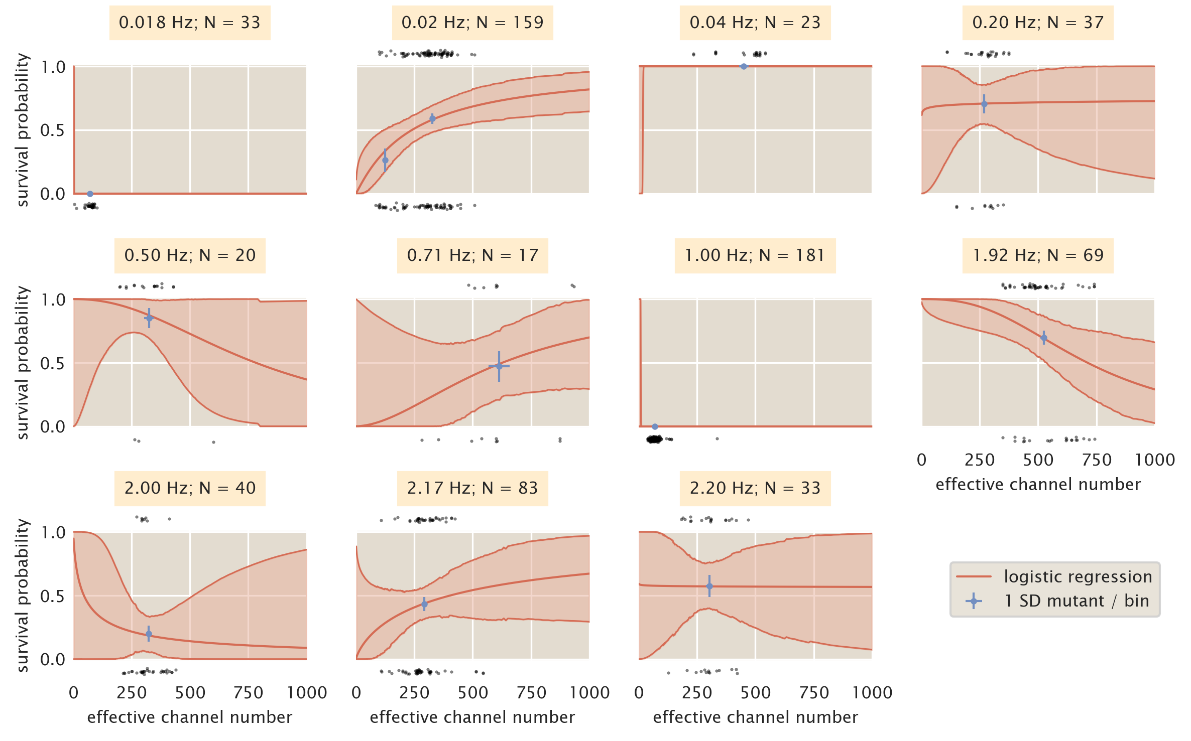
Figure 4: Binning by individual shock rates. Survival probability estimates from logistic regression (red lines) and the computed survival probability for all SD mutants subjected to that shock rate (blue points). Black points at top and bottom of each plot correspond to single cell measurements of survival (top) and death (bottom). Red shaded regions signify the 95% credible region of the logistic regression. Horizontal error bars of blue points are the standard error of the mean channel copy number. Vertical error bars of blue points correspond to the uncertainty in survival probability by observing \(n\) survival events from \(N\) single-cell measurements.
Given the data shown in Fig. 4, we can try to combine the data sets into several bins. Fig. 5 shows the data presented in Fig. 4 separated into "slow" (\(<\) 0.5 Hz, A), "intermediate" (0.5 - 1.0 Hz, B), and "fast" (\(>\) 1.0 Hz, C) shock groups. Using these groupings, the full range of MscL channel copy numbers are covered for each case, with the intermediate shock rate sparsely sampling copy numbers greater than 200 channels per cell. In all three of these cases, the same qualitative story is told -- several hundred channels per cell are necessary for an appreciable level of survival when subjected to an osmotic shock. This argument is strengthened when examining the predicted survival probability by considering all shock rates as a single group, shown in Fig. 5D. This treatment tells nearly the same quantitative and qualitative story as the three rate grouping shown in this section and the two rate grouping presented in the main text. While there does appear to be a dependence on the shock rate for survival when only MscL is expressed, the effect is relatively weak with overlapping credible regions for the logistic regression across the all curves. To account for the sparse sampling of high copy numbers observed in the intermediate shock group, we split this set and partitioned the measurements into either the "slow" (\(<\) 1.0 Hz) or "fast" (\(\geq\) 1.0 Hz) groups presented in the main text of this work.
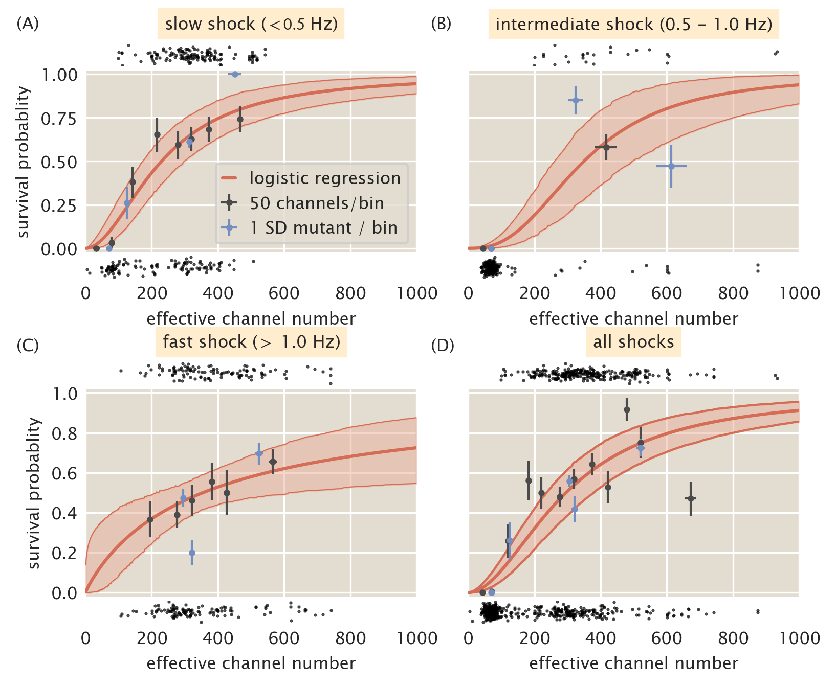
Figure 5: Coarse graining shock rates into different groups. Estimated survival probability curve for slow (A), intermediate (B), and fast (C) shock rates. (D) Estimated survival probability curve from pooling all data together, ignoring varying shock rates. Red shaded regions correspond to the 95% credible region of the survival probability estimated via logistic regression. Black points at top and bottom of each plot represent single-cell measurements of cells which survived and died, respectively. Black points and error bars represent survival probability calculations from bins of 50 channels per cell. Blue points represent the survival probability for a given Shine-Dalgarno mutant. Horizontal error bars are the standard error of the mean with at least 25 measurements and vertical error bars signifies the uncertainty in the survival probability from observing \(n\) survival events out of \(N\) total measurements.
Regression
In this work, we were interested in computing the survival probability under a large hypo-osmotic shock as a function of MscL channel number. As the channel copy number distributions for each Shine-Dalgarno sequence mutant were broad and overlapping, we chose to calculate the survival probability through logistic regression -- a method that requires no binning of the data providing the least biased estimate of survival probability. Logistic regression is a technique that has been used in medical statistics since the late 1950's to describe diverse phenomena such as dose response curves, criminal recidivism, and survival probabilities for patients after treatment (4–6). It has also found much use in machine learning to tune a binary or categorical response given a continuous input (7–9).
In this section, we derive a statistical model for estimating the most-likely values for the coefficients \(\beta_0\) and \(\beta_1\) and use Bayes' theorem to provide an interpretation for the statistical meaning.
Bayesian parameter estimation of \(\beta_0\) and \(\beta_1\)
The central challenge of this work is to estimate the probability of survival \(p_s\) given only a measure of the total number of MscL channels in that cell. In other words, for a given measurement of \(N_c\) channels, we want to know likelihood that a cell would survive an osmotic shock. Using Bayes' theorem, we can write a statistical model for the survival probability as \[ g(p_s\,\vert\, N_c) = {f(N_c\,\vert\, p_s)g(p_s) \over f(N_c)}, \qquad(17)\]
where \(g\) and \(f\) represent probability density functions over parameters and data, respectively. The posterior probability distribution \(g(p_s\,\vert\, N_c)\) describes the probability of \(p_s\) given a specific number of channels \(N_c\). This distribution is dependent on the likelihood of observing \(N_c\) channels assuming a value of \(p_s\) multiplied by all prior knowledge we have about knowing nothing about the data, \(g(s)\). The denominator \(f(N_c)\) in Eq. 17 captures all knowledge we have about the available values of \(N_c\), knowing nothing about the true survival probability. As this term acts as a normalization constant, we will neglect it in the following calculations for convenience.
To begin, we must come up with a statistical model that describes the experimental measurable in our experiment -- survival or death. As this is a binary response, we can consider each measurement as a Bernoulli trial with a probability of success matching our probability of survival \(p_s\), \[ f(s\, \vert\, p_s) = p_s^s(1 - p_s)^{1-s}, \qquad(18)\] where \(s\) is the binary response of \(1\) or \(0\) for survival and death, respectively. As is stated in the introduction to this section, we decided to use a logistic function to describe the survival probability. We assume that the log-odds of survival is linear with respect to the effective channel copy number \(N_c\) as \[ \log{p_s \over 1 - p_s} = \beta_0 + \beta_1 N_c, \qquad(19)\] where \(\beta_0\) and \(\beta_1\) are coefficients which describe the survival probability in the absence of channels and the increase in log-odds of survival conveyed by a single channel. The rationale behind this interpretation is presented in the following section, A Bayesian interpretation of \(\beta_0\) and \(\beta_1\). Using this assumption, we can solve for the survival probability \(p_s\) as, \[ p_s = {1 \over 1 + e^{-\beta_0 -\beta_1 N_c}}. \qquad(20)\]
With a functional form for the survival probability, the likelihood stated in Eq. 17 can be restated as \[ f(N_c, s\,\vert\,\beta_0,\beta_1) = \left({1 \over 1 + e^{-\beta_0 - \beta_1 N_c}}\right)^s\left(1 - {1 \over 1 + e^{-\beta_0 - \beta_1 N_c}}\right)^{1 - s}. \qquad(21)\] As we have now introduced two parameters, \(\beta_0\), and \(\beta_1\), we must provide some description of our prior knowledge regarding their values. As is typically the case, we know nothing about the values for \(\beta_0\) and \(\beta_1\). These parameters are allowed to take any value, so long as it is a real number. Since all values are allowable, we can assume a flat distribution where any value has an equally likely probability. This value of this constant probability is not necessary for our calculation and is ignored. For a set of \(k\) single-cell measurements, we can write the posterior probability distribution stated in Eq. 17 as \[ g(\beta_0, \beta_1\,\vert\, N_c, s) = \prod\limits_{i=1}^n\left({1 \over 1 + e^{-\beta_0 - \beta_1 N_c^{(i)}}}\right)^{s^{(i)}}\left(1 - {1 \over 1 + e^{-\beta_0 - \beta_1 N_c^{(i)}}}\right)^{1 - s^{(i)}} \qquad(22)\]
Implicitly stated in Eq. 22 is absolute knowledge of the channel copy number \(N_c\). However, as is described in Standard Candle Calibration, we must convert from a measured areal sfGFP intensity \(I_A\) to a effective channel copy number, \[ N_c = {I_A \tilde{\langle A \rangle} \over \tilde{\alpha}}, \qquad(23)\] where \(\tilde{\langle A \rangle}\) is the average cell area of the standard candle strain and \(\tilde{\alpha}\) is the most-likely value for the calibration factor between arbitrary units and protein copy number. In Standard Candle Calibration, we detailed a process for generating an estimate for the most-likely value of \(\tilde{\langle A \rangle}\) and \(\tilde{\alpha}\). Given these estimates, we can include an informative prior for each value. From the Markov chain Monte Carlo samples shown in Fig. 2, the posterior distribution for each parameter is approximately Gaussian. By approximating them as Gaussian distributions, we can assign an informative prior for each as \[ g(\alpha\,\vert\,\tilde{\alpha}, \tilde{\sigma}_\alpha) \propto {1 \over \tilde{\sigma}_\alpha^k}\prod\limits_{i=1}^k\exp\left[-{(\alpha_i - \tilde{\alpha})^2 \over 2\tilde{\sigma}_\alpha^2}\right] \qquad(24)\] for the calibration factor for each cell and \[ g(\langle A \rangle\,\vert\,\tilde{\langle A \rangle},\tilde{\sigma}_{\langle A \rangle}) = {1 \over \tilde{\sigma}_{\langle A \rangle}^k}\prod\limits_{i=1}^k\exp\left[-{(\langle A \rangle_i - \tilde{\langle A \rangle})^2 \over 2\tilde{\sigma}_{\langle A \rangle}^2}\right], \qquad(25)\] where \(\tilde{\sigma}_\alpha\) and \(\tilde{\sigma}_{\langle A \rangle}\) represent the variance from approximating each posterior as a Gaussian. The proportionality for each prior arises from the neglecting of normalization constants for notational convenience.
Given Eq. 21 through Eq. 25, the complete posterior distribution for estimating the most likely values of \(\beta_0\) and \(\beta_1\) can be written as \[ \begin{aligned} g(\beta_0, &\beta_1\,\vert\,[I_A, s],\tilde{\langle A \rangle}, \tilde{\sigma}_{\langle A \rangle}, \tilde{\alpha}, \tilde{\sigma}_\alpha) \propto{1 \over (\tilde{\sigma}_\alpha\tilde{\sigma}_{\langle A \rangle})^k}\prod\limits_{i=1}^k\left(1 + \exp\left[-\beta_0 - \beta_1 {{I_A}_i \langle A \rangle_i \over \alpha_i}\right]\right)^{-s_i}\,\times\,\\ &\left(1 - \left(1 + \exp\left[-\beta_0 - \beta_1 {{I_A}_i\langle A \rangle_i \over \alpha_i}\right]\right)^{-1}\right)^{1 - s_i} \exp\left[-{(\langle A \rangle_i - \tilde{\langle A \rangle})^2 \over 2\tilde{\sigma}_{\langle A \rangle}} - {(\alpha_i - \tilde{\alpha})^2\over 2\tilde{\sigma}_\alpha^2}\right] \end{aligned}. \qquad(26)\]
As this posterior distribution is not solvable analytically, we used Markov chain Monte Carlo to draw samples out of this distribution, using the log of the effective channel number as described in the main text. The posterior distributions for \(\beta_0\) and \(\beta_1\) for both slow and fast shock rate data can be seen in Fig. 6
Figure 6: Posterior distributions for logistic regression coefficients evaluated for fast and slow shock rates. (A) Kernel density estimates of the posterior distribution for \(\beta_0\) for fast (blue) and slow (purple) shock rates. (B) Kernel density estimates of posterior distribution for \(\beta_1\).
A Bayesian interpretation of \(\beta_0\) and \(\beta_1\)
The assumption of a linear relationship between the log-odds of survival and the predictor variable \(N_c\) appears to be arbitrary and is presented without justification. However, this relationship is directly connected to the manner in which Bayes' theorem updates the posterior probability distribution upon the observation of new data. In following section, we will demonstrate this connection using the relationship between survival and channel copy number. However, this description is general and can be applied to any logistic regression model so long as the response variable is binary. This connection was shown briefly by Allen Downey in 2014 and has been expanded upon in this work (10).
The probability of observing a survival event \(s\) given a measurement of \(N_c\) channels can be stated using Bayes' theorem as \[ g(s\,\vert\, N_c) = {f(N_c\,\vert\, s)g(s) \over f(N_c)}. \qquad(27)\] where \(g\) and \(f\) represent probability density functions over parameters and data respectively. The posterior distribution \(g(s\,\vert\, N_c)\) is the quantity of interest and implicitly related to the probability of survival. The likelihood \(g(N_c\,\vert\, s)\) tells us the probability of observing \(N_c\) channels in this cell given that it survives. The quantity \(g(s)\) captures all a priori knowledge we have regarding the probability of this cell surviving and the denominator \(f(N_c)\) tells us the converse -- the probability of observing \(N_c\) cells irrespective of the survival outcome.
Proper calculation of Eq. 27 requires that we have knowledge of \(f(N_c)\), which is difficult to estimate. While we are able to give appropriate bounds on this term, such as a requirement of positivity and some knowledge of the maximum membrane packing density, it is not so obvious to determine the distribution between these bounds. Given this difficulty, it's easier to compute the odds of survival \(\mathcal{O}(s\,\vert\, N_c)\), the probability of survival \(s\) relative to death \(d\), \[ \mathcal{O}(s\,\vert\, N_c) = {g(s\,\vert\,N_c) \over g(d\,\vert\, N_c)} = {f(N_c\,\vert\, s)g(s) \over f(N_c\,\vert\,d)g(d)}, \qquad(28)\] where \(f(N_c)\) is cancelled. The only stipulation on the possible value of the odds is that it must be a positive value. As we would like to equally weigh odds less than one as those of several hundred or thousand, it is more convenient to compute the log-odds, given as \[ \log \mathcal{O}(s\,\vert\,N_c)= \log {g(s) \over g(d)} + \log {f(N_c \,\vert\, s )\over f(N_c\,\vert\, d)}. \qquad(29)\] Computing the log-transform reveals two interesting quantities. The first term is the ratio of the priors and tells us the a priori knowledge of the odds of survival irrespective of the number of channels. As we have no reason to think that survival is more likely than death, this ratio goes to unity. The second term is the log likelihood ratio and tells us how likely we are to observe a given channel copy number \(N_c\) given the cell survives relative to when it dies.
For each channel copy number, we can evaluate Eq. 29 to measure the log-odds of survival. If we start with zero channels per cell, we can write the log-odds of survival as \[ \log \mathcal{O}(s\,\vert\,N_c=0) = \log {g(s) \over g(d)} + \log {f(N_c=0\,\vert\, s) \over f(N_c=0\,\vert\, d)}. \qquad(30)\] For a channel copy number of one, the odds of survival is \[ \log \mathcal{O}(s\,\vert\,N_c=1) = \log{g(s) \over g(d)} + \log{f(N_c=1\,\vert\, s) \over f(N_c=1\,\vert\, d)}. \qquad(31)\] In both Eq. 30 and Eq. 31, the log of our a priori knowledge of survival versus death remains. The only factor that is changing is log likelihood ratio. We can be more general in our language and say that the log-odds of survival is increased by the difference in the log-odds conveyed by addition of a single channel. We can rewrite the log likelihood ratio in a more general form as \[ \log {f(N_c\, \vert\, s) \over f(N_c\,\vert\, d)} = \log{f(N_c = 0\,\vert\,s) \over f(N_c=0\,\vert\, d)} + N_c \left[\log{f(N_c=1 \,\vert\,s) \over f(N_c=1\,\vert\, d)} - \log{f(N_c=0\,\vert\, s) \over f(N_c=0\,\vert\, d)}\right], \qquad(32)\] where we are now only considering the case in which \(N_c \in [0, 1]\). The bracketed term in Eq. 32 is the log of the odds of survival given a single channel relative to the odds of survival given no channels. Mathematically, this odds-ratio can be expressed as \[ \log\mathcal{OR}_{N_c}(s) = \log{{f(N_c=1\,\vert\,s)g(s)\over f(N_c=1\,\vert\,d)g(d)}\over {f(N_c=0\,\vert\,s)g(s)\over f(N_c=0\,\vert\,d)g(d)}} = \log{f(N_c=1\,\vert\,s) \over f(N_c=1\,\vert\,d)} - \log{f(N_c=0\,\vert\,s)\over f(N_c=0\,\vert\,d)} . \qquad(33)\] Eq. 33 is mathematically equivalent to the bracketed term shown in Eq. 32.
We can now begin to staple these pieces together to arrive at an expression for the log odds of survival. Combining Eq. 32 with Eq. 29 yields \[ \log \mathcal{O}(s\,\vert\,N_c) = \log{g(s) \over g(d)} + \log {f(N_c=0\,\vert\, s) \over f(N_c=0\,\vert\, d)} + N_c\left[{f(N_c=1\,\vert\,s)\over f(N_c=1\,\vert\,d)} - \log{f(N_c=0\,\vert\,s) \over f(N_c=0\,\vert\,d)}\right]. \qquad(34)\] Using our knowledge that the bracketed term is the log odds-ratio and the first two times represents the log-odds of survival with \(N_c=0\), we conclude with \[ \log\mathcal{O}(s\,\vert\,N_c) = \log \mathcal{O}(s\,\vert\,N_c=0) + N_c \log \mathcal{OR}_{N_c}(s). \qquad(35)\] This result can be directly compared to Eq. 1 presented in the main text, \[ \log {p_s \over 1 - p_s} = \beta_0 + \beta_1 N_c, \qquad(36)\] which allows for an interpretation of the seemingly arbitrary coefficients \(\beta_0\) and \(\beta_1\). The intercept term, \(\beta_0\), captures the log-odds of survival with no MscL channels. The slope, \(\beta_1\), describes the log odds-ratio of survival which a single channel relative to the odds of survival with no channels at all. While we have examined this considering only two possible channel copy numbers (\(1\) and \(0\)), the relationship between them is linear. We can therefore generalize this for any MscL copy number as the increase in the log-odds of survival is constant for addition of a single channel.
Other properties as predictor variables
The previous two sections discuss in detail the logic and practice behind the application of logistic regression to cell survival data using only the effective channel copy number as the predictor of survival. However, there are a variety of properties that could rightly be used as predictor variables, such as cell area and shock rate. As is stipulated in our standard candle calibration, there should be no correlation between survival and cell area. Fig. 7A and B show the logistic regression performed on the cell area. We see for both slow and fast shock groups,there is little change in survival probability with changing cell area and the wide credible regions allow for both positive and negative correlation between survival and area. The appearance of a bottle neck in the notably wide credible regions is a result of a large fraction of the measurements being tightly distributed about a mean value. Fig. 7C shows the predicted survival probability as a function of the the shock rate. There is a slight decrease in survivability as a function of increasing shock rate, however the width of the credible region allows for slightly positive or slightly negative correlation. While we have presented logistic regression in this section as a one-dimensional method, Eq. 19 can be generalized to \(n\) predictor variables \(x\) as \[ \log {p_s \over 1 - p_s} = \beta_0 + \sum\limits_{i}^n \beta_ix_i. \qquad(37)\] Using this generalization, we can use both shock rate and the effective channel copy number as predictor variables. The resulting two-dimensional surface of survival probability is shown in Fig. 7D. As is suggested by Fig. 7C, the magnitude of change in survivability as the shock rate is increased is smaller than that along increasing channel copy number, supporting our conclusion that for MscL alone, the copy number is the most important variable in determining survival.
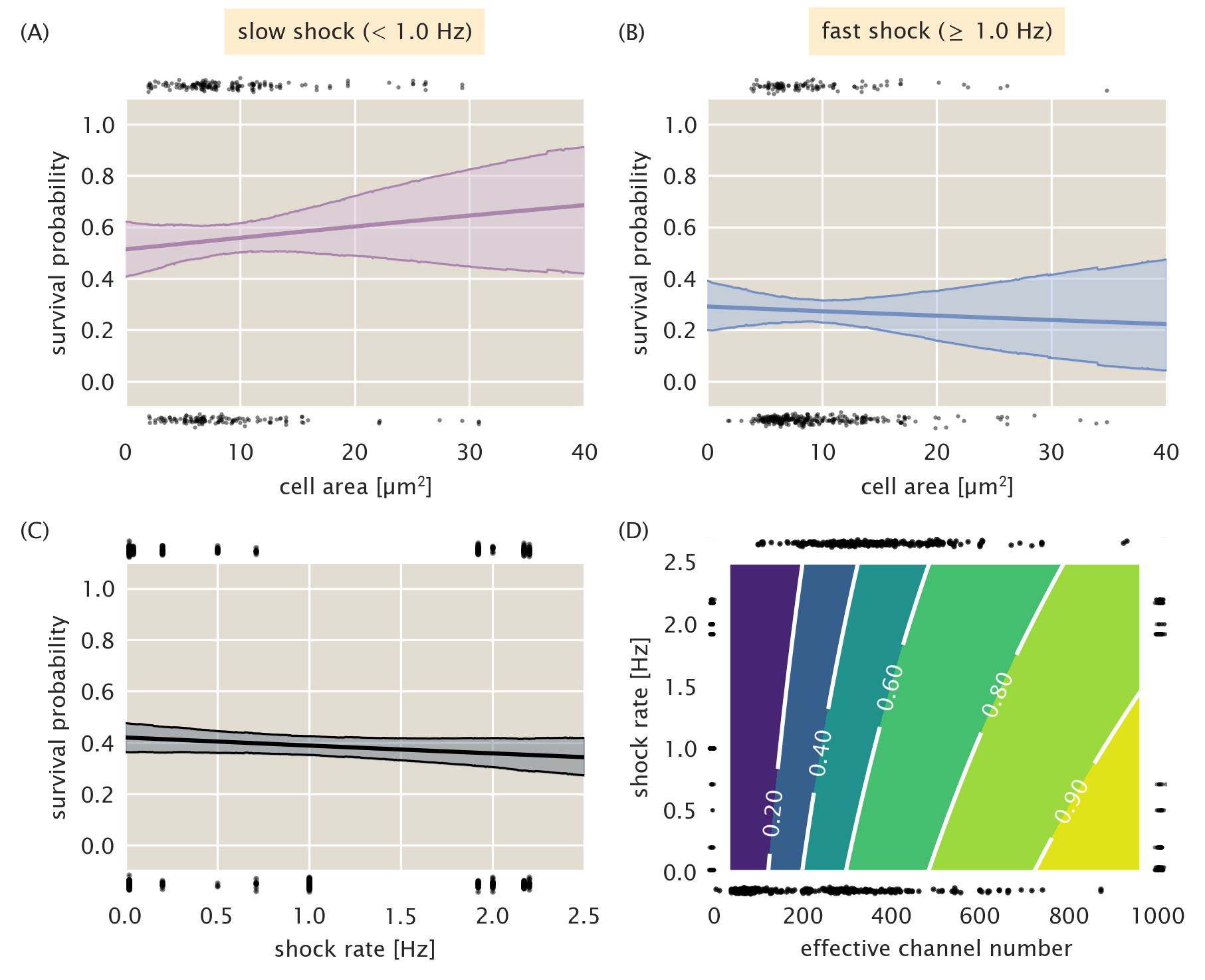
Figure 7: Survival probability estimation using alternative predictor variables. (A) Estimated survival probability as a function of cell area for the slow shock group. (B) Estimated survival probability as a function of cell area for the fast shock group. (C) Estimated survival probability as a function shock rate. Black points at top and bottom of plots represent single-cell measurements of cells who survived and perished, respectively. Shaded regions in (A) - (C) represent the 95% credible region. (D) Surface of estimated survival probability using both shock rate and effective channel number as predictor variables. Black points at left and right of plot represent single-cell measurements of cells which survived and died, respectively, sorted by shock rate. Points at top and bottom of plot represent survival and death sorted by their effective channel copy number. Labeled contours correspond to the survival probability.
| Strain name | Genotype | Reference |
|---|---|---|
| MJF641 | Frag1, \(\Delta\)mscL::cm, \(\Delta\)mscS, \(\Delta\)mscK::kan, \(\Delta\)ybdG::apr, \(\Delta\)ynaI, \(\Delta\)yjeP, \(\Delta\)ybiO, ycjM::Tn10 | (11) |
| MLG910 | MG1655, \(\Delta\)mscL ::\(\phi\)mscL-sfGFP, \(\Delta\)galK::kan, \(\Delta\)lacI, \(\Delta\)lacZY A | (1) |
| D6LG-Tn10 | Frag1, \(\Delta\)mscL ::\(\phi\)mscL-sfGFP, \(\Delta\)mscS, \(\Delta\)mscK::kan, \(\Delta\)ybdG::apr, \(\Delta\)ynaI, \(\Delta\)yjeP, \(\Delta\)ybiO, ycjM::Tn10 | This work |
| D6LG (SD0) | Frag1, \(\Delta\)mscL ::\(\phi\)mscL-sfGFP, \(\Delta\)mscS, \(\Delta\)mscK::kan, \(\Delta\)ybdG::apr, \(\Delta\)ynaI, \(\Delta\)yjeP, \(\Delta\)ybiO | This work |
| XTL298 | CC4231, araD:: tetA-sacB-amp | (12) |
| D6LTetSac | Frag1, mscL-sfGFP:: tetA-sacB, \(\Delta\)mscS, \(\Delta\)mscK::kan, \(\Delta\)ybdG::apr, \(\Delta\)ynaI, \(\Delta\)yjeP, \(\Delta\)ybiO | This work |
| D6LG (SD1) | Frag1, \(\Delta\)mscL ::\(\phi\)mscL-sfGFP, \(\Delta\)mscS, \(\Delta\)mscK::kan, \(\Delta\)ybdG::apr, \(\Delta\)ynaI, \(\Delta\)yjeP, \(\Delta\)ybiO | This work |
| D6LG (SD2) | Frag1, \(\Delta\)mscL ::\(\phi\)mscL-sfGFP, \(\Delta\)mscS, \(\Delta\)mscK::kan, \(\Delta\)ybdG::apr, \(\Delta\)ynaI, \(\Delta\)yjeP, \(\Delta\)ybiO | This work |
| D6LG (SD4) | Frag1, \(\Delta\)mscL ::\(\phi\)mscL-sfGFP, \(\Delta\)mscS, \(\Delta\)mscK::kan, \(\Delta\)ybdG::apr, \(\Delta\)ynaI, \(\Delta\)yjeP, \(\Delta\)ybiO | This work |
| D6LG (SD6) | Frag1, \(\Delta\)mscL ::\(\phi\)mscL-sfGFP, \(\Delta\)mscS, \(\Delta\)mscK::kan, \(\Delta\)ybdG::apr, \(\Delta\)ynaI, \(\Delta\)yjeP, \(\Delta\)ybiO | This work |
| D6LG (12SD2) | Frag1, \(\Delta\)mscL ::\(\phi\)mscL-sfGFP, \(\Delta\)mscS, \(\Delta\)mscK::kan, \(\Delta\)ybdG::apr, \(\Delta\)ynaI, \(\Delta\)yjeP, \(\Delta\)ybiO | This work |
| D6LG (16SD0) | Frag1, \(\Delta\)mscL ::\(\phi\)mscL-sfGFP, \(\Delta\)mscS, \(\Delta\)mscK::kan, \(\Delta\)ybdG::apr, \(\Delta\)ynaI, \(\Delta\)yjeP, \(\Delta\)ybiO | This work |
| Primer Name | Sequence (5' \(\rightarrow\) 3') |
|---|---|
| Tn10delR | taaagccaacggcatccaggcggacatactcagca|| |
cctttcgcaaggtaacagagtaaaacatccaccat |
|
| MscLSPSac | gaaaatggcttaacatttgttagacttatggttgtcgg |
cttcatagggagTCCTAATTTTTGTTGACACTCTATC |
|
| MscLSPSacR | accacgttcccgcgcatcgcaaattcgcgaaat |
tctttaataatgctcatATCAAAGGGAAAACTGTCCATA |
|
| MscL-SD1R | atcgcaaattcgcgaaattctttaataatgctcat |
gttattctcctcatgaagccgacaaccataagtctaacaaa |
|
| MscL-SD2R | atcgcaaattcgcgaaattctttaataatgctcatgttatt |
tcccctatgaagccgacaaccataagtctaacaaa |
|
| MscL-SD4R | atcgcaaattcgcgaaattctttaataatgctcat |
gttatt cctgctatgaagccgacaaccataagtctaacaaa |
|
| MscL-SD6R | atcgcaaattcgcgaaattctttaataatgctcat |
gttatt gctcgtatgaagccgacaaccataagtctaacaaa |
|
| MscL-12SD2R | atcgcaaattcgcgaaattctttaataatgctcat |
atatatatatat tcccctatgaagccgacaaccataagtctaacaaa |
|
| MscL-16SD0R | atcgcaaattcgcgaaattctttaataatgctcat |
atatatatatatatat ctccctatgaagccgacaaccataagtctaacaaa |
Strains
1. Bialecka-Fornal M, Lee HJ, DeBerg HA, Gandhi CS, Phillips R. 2012. Single-Cell Census of Mechanosensitive Channels in Living Bacteria. PLoS ONE 7:e33077.
2. Sivia D, Skilling J. 2006. Data Analysis: A Bayesian TutorialSecond Edition. Oxford University Press, Oxford, New York.
3. Bialecka-Fornal M, Lee HJ, Phillips R. 2015. The Rate of Osmotic Downshock Determines the Survival Probability of Bacterial Mechanosensitive Channel Mutants. Journal of Bacteriology 197:231–237.
4. Anderson RP, Jin R, Grunkemeier GL. 2003. Understanding logistic regression analysis in clinical reports: An introduction. The Annals of Thoracic Surgery 75:753–757.
5. Mishra V, Skotak M, Schuetz H, Heller A, Haorah J, Chandra N. 2016. Primary blast causes mild, moderate, severe and lethal TBI with increasing blast overpressures: Experimental rat injury model. Scientific Reports 6:26992.
6. Stahler GJ, Mennis J, Belenko S, Welsh WN, Hiller ML, Zajac G. 2013. Predicting Recidivism For Released State Prison Offenders. Criminal justice and behavior 40:690–711.
7. Cheng W, Hüllermeier E. 2009. Combining instance-based learning and logistic regression for multilabel classification. Machine Learning 76:211–225.
8. Dreiseitl S, Ohno-Machado L. 2002. Logistic regression and artificial neural network classification models: A methodology review. Journal of Biomedical Informatics 35:352–359.
9. Ng AY, Jordan MI. On Discriminative vs. Generative Classifiers: A comparison of logistic regression and naive Bayes 8.
10. Downey A. 2014. Probably Overthinking It: Bayes’s theorem and logistic regression. Probably Overthinking It.
11. Edwards MD, Black S, Rasmussen T, Rasmussen A, Stokes NR, Stephen TL, Miller S, Booth IR. Jul-Aug 20122012. Characterization of three novel mechanosensitive channel activities in Escherichia coli. Channels (Austin) 6:272–81.
12. Li X-t, Thomason LC, Sawitzke JA, Costantino N, Court DL. 2013. Positive and negative selection using the tetA-sacB cassette: Recombineering and P1 transduction in Escherichia coli. Nucleic acids research 41:e204–e204.